1. INTRODUCTION
One of the main objectives in analyzing data is to learn from past events and to incorporate this knowledge for future planning and decision-making. This involves the use of all the current and past information to forecast future outcomes. In forecasting, the time horizon is determined by the characteristic timescales of the process concerned and the objective in exercising the analysis. For example, the scheduling of production and inventories requires short-term forecasts while longer horizons are required when the long-term prospect ranging from expansions in a plant to environmental factor impacts is investigated (Niu and Harris, 1996; Kwon et al., 2002). Typical periods in the first case are 10–14 weeks and 3–5 years and more for the second.
The problem of short-term forecasting has been addressed extensively in the past. A detailed review of various short-term forecasting models can be found in Harvey (1984). However, long-term forecasting, from a practical viewpoint, is considered more qualitative in nature involving both the forecasters’ skills and the available information on an ad hoc basis, has suggested by Kendall and Ord (1993), Armstrong (1985), and Martino (1983). Research on theoretical aspects of long-term forecasting models has covered various modifications of short-term forecasting models. Kabaila (1981), Stoica and Soderstorm (1984), and Tiao and Xu (1993) have suggested different least square parameter estimates of the one-step ahead forecasting model to incorporate multiple steps ahead predictions. Different Box Jenkins models have been suggested by Findley (1983), Gersch and Kitagawa (1983), and Lin and Granger (1994). Furthermore, Pillai (1992) has used the maximum entropy criterion for multistep predictions. Other strategies include the direct “plug-in” method where unobserved values are successively replaced by their one-step ahead forecasts. Bhansali (1996, 1999) has provided theoretical grounds for the optimality in using a single model for multiple steps ahead forecasting while Kang (2003) has suggested the use of different models for different spans of the process under investigation.
In general, the possibility of incorporating different horizons forecasts requires the study of two types of variation. These are the inherent structural variation that characterizes the long term nature of the process and the short-term high-frequency variation. The existing short (long) term forecasting models are not designed to separate these characteristics, and therefore, not reliable in generating long (short) term forecasts.
In this paper, a new approach is introduced in which the characteristics of different variational parameters are preserved making forecasting over different horizons possible in a logical manner.
The close link between autoregressive integrated moving averages (ARIMA) and the state space representation is explained in both the statistical and control engineering literature (Box and Jenkins, 1970; Anderson and Moore, 1979).
Assuming that {Yt|q1,t} is a time series process with the parameter vector q1,trepresenting the state of the process, a dynamic linear model (DLM) is shown in the Equation (1):

And, the state transition is calculated in Equation (2):

Where F1,t, and G1,t are known, and {Jt} and {ωt} are uncorrelated normal variates with zero means.
This has been extended to model correlated variables by adding a third Equation (3) representing transitions on vt so that:

Where G2 is assumed known and εt is a normal variate with zero mean vector (Anderson and Moor 1979. p. 290). However, the model can be reparametrized as a non-linear predictor model (NPM), Ameen (1992), in which the autoregressive components, G2, can be assumed known and updated through time.
A main drawback of linear structures in modeling correlated observations is that information is filtered between different state parameter components using the usual Kalman filter. The underlying parameters are updated according to a common one-step forecasting error. This makes causal model parameters to lose their characteristic properties during the sequential updating process. For example, it is not possible to consider one-step forecasting errors that are calculated from a short term model for the parameters identifying long term structures and vice versa. This may suggest that the two characteristics are separable and independent modeling structures should be implemented. Earlier efforts have been concentrated on the idea of curve fitting. Gregg et al. (1964) and later Harrison and Pearce (1972) have presented comprehensive accounts of the ICI methodology for long-term forecasting. These authors have discussed extrapolation techniques using some specific functions as trend curves. More discussions on these curves and confidence limits on forecasts can be found in the study of Levenbach and Reuter (1976). Harrison et al. (1977) have constructed models that consider randomness around predetermined linear/non-linear global trends all constructed to provide long-term forecasts. Although there is a logical connection between forecasts for different horizons, lead time periods separating short-, medium-, and long-term forecasts are rather subjective and difficult to justify.
The discounting principle of Ameen and Harrison (1985) has extensively been used in Bayesian modeling and forecasting (Harrison and Akram, 1983; Migon and Harrison, 1985). In these models, low frequencies are modeled using autoregressive parameters. Although this can accommodate the correlation between the departures from the underlying trend, the identification and estimation of many autoregressive parameters can be tedious. Moreover, different model parameter updates are dominated by one source of information (one-step forecasting errors). The models have no facilities to encapsulate the long-and short-term behavior of the time series. More recently, Danesiet al. (2017) have followed a form of variability decomposition (Al-Madfai, 2002; Al-Madfaiet al., 2004) extracting some underlying smooth function to capture the long-term behavior of the time series in question and adopt the ARIMA modeling technique on the remainder.
This paper is an attempt to resolve these problems by introducing a fairly general method in which characteristic properties of different state parameter vectors are preserved in updating. This is performed using the idea of submodels. The problem of identification and estimation of autoregressive parameters is overcome through the introduction of a set of easily assessed discount factors. Although the idea is fairly general, we concentrate on the case of normality with random level and growth components. Generalizations to higher dimensions follow easily. The general idea is presented in Section 2 in which full recursive formulas for parameter estimates are given. A number of limiting properties are discussed, and models structural behavior and limiting forecast functions are given in Section 3.
Throughout this paper, X ~ N[a; b] means that X is normally distributed with mean a and variance b. The same holds for random vectors.
2. LOCAL AND GLOBAL FORECASTING MODELS
Let, {Yt|qt} be a process with low- and high-frequency variations. Furthermore, assume that these variations are represented by q1,t and q2,t as the components of qt, respectively. Furthermore, let M1 and M2 be subjects modeling the existing low- and high-frequency parameters, respectively. In the above, the parameter vector q1,t may be identifying a general polynomial trend approximating the inherent underlying process structure while q2,t may represent the causal variability around that of q1,t.
The common approach for modelling such scenarios has been through the specification of an observation probability distribution f(yt|q1,t, q2,t) accompanied by a prior state distribution f(q1,t, q2,t|Dt−1, M1, M2) where Dt−1 represents the information available at time t−1 including past observations. A before posterior transition in time together with the above specifications allows a complete Bayesian sequential estimation to be conducted for the estimation of model parameters. The general DLMs of Harrison and Stevens (1976) and NPM of Ameen (1992) are examples of such kind. The broad specification above contains both the high and low dimensionalities of the process in a combined form. As a result, the defined models do not allow the two parameter vectors q1,t and q2,t to preserve their characteristics as they are both updated using one error structure. In such cases, a joint forecasting distribution seems inadequate as the updating structure for q1,t and q2,t remains less informative about the short- or long-term behavior of the process.
The two types of variability discussed above are conditionally independent. That is, given the observation yt, q1,t is independent on q2,tand this can be exploited to learn about these parameters in one model. The resulting model can be used to bridge the gap between forecasts for different horizons and make data analysis more efficient in some practical cases.
The practical need for estimating parameters of different characteristics has led by Smith et al. (1994) to construct a two-stage sales forecasting procedure using discounted least squares. The low-frequency variations are modelled in one stage followed by the modeling of the departures from this trend as a second stage.
Using the above terminology, we have the following Equation (4):

Moreover, the general forecast function may be expressed as follows:
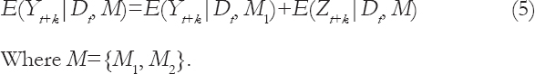
Where M={M1,M2}
Furthermore, the departures Zt are modelled so that E{Zt+k|Dt, M} → 0 as k → ∞. This property ensures a logical transition between forecasts for different horizons from a single model as the lead-time increases.
The underlying modeling strategy is described as follows:
Given the observation distribution:

And, posterior distributions at time t−1:
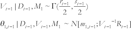
The prior distributions for time t are defined as follows:
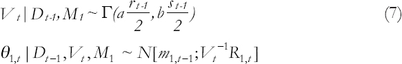
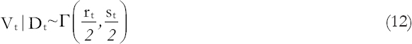
Where
And, β1< 1 is a discount factor with a value subjectively selected to be close to 1. The constants a and b are introduced to accommodate trends in the evolution of the likelihood variance since E(Vt|Dt−1) = art−1/bst−1.
The above model incorporates correlated inputs and can be extended to multiple discount factors as necessary (Ameen and Harrison, 1985; Ameen, 1992 for more elaboration on the choice of the discount factor and the constants a and b). A sequential updating procedure is then obtained representing the evolution of the low-frequency parameters with time.
The resulting forecasting distribution is as follows:

Where


The posterior state distribution for time t is as follows:

Where
Moreover, the updated variance distribution is as follows:
Where

Note that, all the above distributions that are conditional on Vt, their unconditional distributions can be found using the rules of probability leading to t-distributions with appropriate parameter values.
Alternatively, Vtvalues can be replaced by their estimates keeping the distributions normal.
Now, given the joint likelihood for the high and low frequencies as:

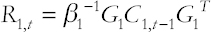
Where the V2,t’s are all uncorrelated, the information in the Equation (6) and Equation (11) can be used to construct the posterior distribution for the high-frequency system parameter vector q2,t−1:

Where m2,t−1=E{q2,t−1|M, Dt−1} and Pt−1 is a known m×n matrix similar to the usual regression coefficients and whose components are functions of the adaptive factors.
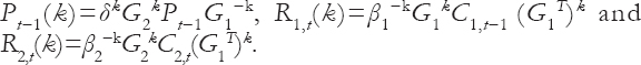
The prior conditional distribution for q2,tis as follows:

Where P*t−1 is obtained from Pt−1 to reflect the added degree of uncertainty due to the transition in time. For example, a direct calculation based on the normal discount Bayesian models setting of Ameen and Harrison (1985) leads to P*t−1=δG2Pt−1G1−1, where δ=(β2/β1)1/2 and R2,t is obtained using the discount principle described earlier. The discount factor β2 is similar to β1 but smaller in magnitude to increase the adaptivity for the estimation of high-frequency parameters.
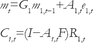
Combining the Equation (13) and Equation (15) and using Bayes theorem, the updating conditional distribution of q2,t is obtained.

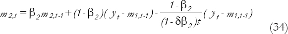
Where


And,

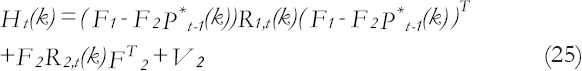
The forecast distribution is given by

Where

And,
The general k steps forecast function is given by

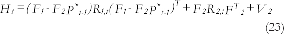
With a forecasting variance of
Where
In practice, G2 can be selected so that G2k→ 0 for large values of k so that the limiting forecast function

3. LIMITING RESULTS
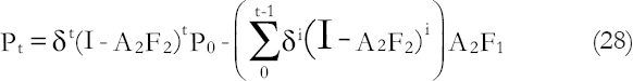
Given that, the eigenvalues of β1G1 and β2G2 are outside the unit circle, it can be seen that (Ameen and Harrison, 1985)

Given a posterior to prior transition for Pt−1 so that P*t−1=δPt−1 where δ≤1 is a known constant, we have Equation (28).


To discuss the limiting predictor functions described here, three simple but rather popular model settings are considered.
3.1. The Steady State M2 and a Static Regression M1Submodel
This restricts the models to scalar forms with F1=F2=G1=G2=β1=1 and δ and β2 are as before.
Therefore, under M1,
And,

It can also be seen which gives
And, as t increases,

That is, the short-term departures are the exponentially weighted moving average (EWMA) of the past departures of the long-term predictions from the observed values.
The k-steps forecasting function is as follows:

Clearly, as k increases, the k-steps forecast function approaches the mean value of Y at time t.
3.2. The Steady State M1 and a Steady State M2Submodel
This restricts the models to scalar forms with F1=F2=G1=G2=1, and β1, δ, and β2 are as before.
Under this formulation, Ai=1−βi, i=1, 2 and P = −(1−β2)/(1−δβ2).
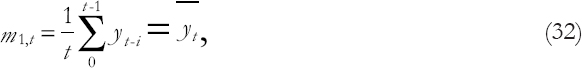
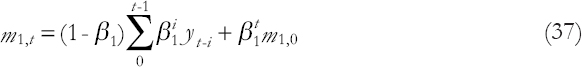
Furthermore, under M1, the low-frequency state parameter is the EWMA of the past observations:
While the high-frequency parameter estimate is
The k-steps forecasting function is:


3.3. Linear Growth M1 and a Steady State M2Submodel
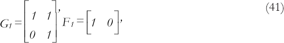
This defines β1, β2, G2, and F2 as in example (i) and

With the limiting adaptive coefficients are as follows:

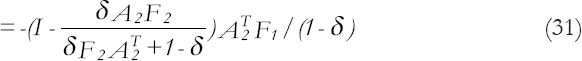
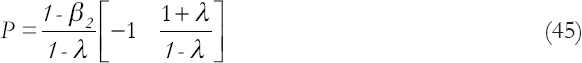
And, also using the relation

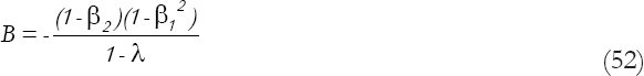
Where λ=β2δ, the limiting Pt can be found as

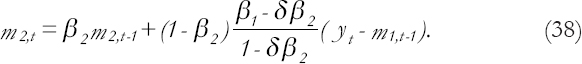
The limiting short-term systems parameter is then updated according to the departures from the estimated trend under M1.
Or

Where

The k-steps forecasting function is:

Furthermore, with a diminishing prior-posterior regression coefficients matrix Pt such that

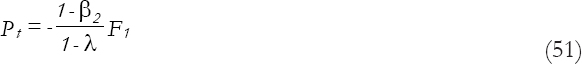
Leading to a modification in the above recurrence relation with